
Hey there, to begin with
in general, Are you a beginner, who started learning a DSP programming and find the hardest part in the DSP programming is coming up with DSP algorithms to create a new project
as a matter of fact, in order develop DSP algorithms we used C language and Gnuplot tool to plot signals
at this time, let’s start with developing the algorithm for signal mean-variance, and standard deviation
Before we automate a code for signal mean let’s first understand what is mean
Signal mean
in a word, signal Mean is the average value of a signal
that is, Mean =  (mu)
(mu)
(1) 
Where
n: is total no of samples
n-1: represents the amplitude
on this occasion, in order to calculate Mean, we simply sum up all the amplitudes of a signal and divide by total no of samples
![\[ \mu=\frac{X_0+X_1+X_2+X_3+X_4......+X_n-1}{n} \]](https://aneescraftsmanship.com/wp-content/ql-cache/quicklatex.com-13e3aad988a6a965c873d6bb97148232_l3.png "Rendered by QuickLaTeX.com")
in essence, for building the logic consider a simple example
in short, Mean= Add all the values/no of values
=(10+20+30+40+45+50+60)/7
=255/7
=36.42
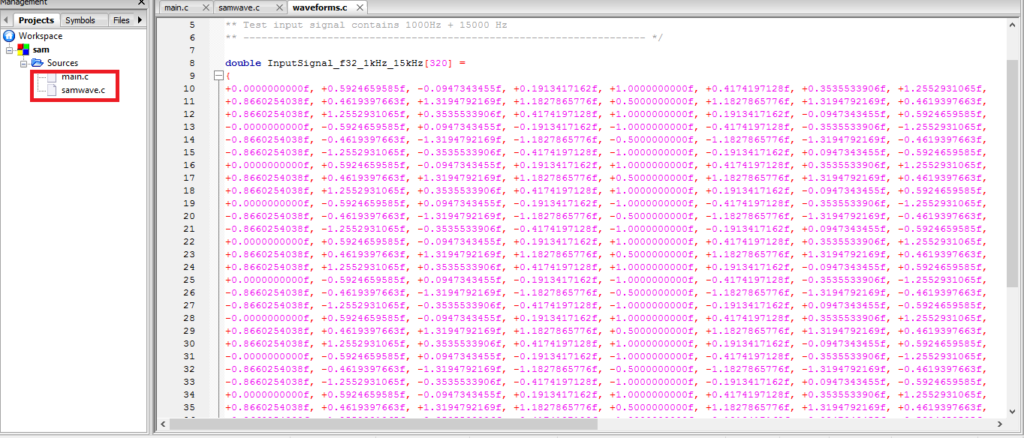
not to mention, to develop signal mean algorithm we used signal source from here —>, you just need to import this file into your main.c file
on the whole, the source signal is generated in Matlab
in the first place, do you know, How to import external file in code block ide?
If not, Then let me guide you, how you can import external file and link it to the main function
- Open code block
- Create a new project—->console application—->Go—->C
- Next —->project name—->next
- On the left side click sources (+) symbol then select main.c
- Write the main program
- Now click on file—->new—->new—->empty file
- ADD file to project
#include <stdio.h>
#include <stdlib.h>
#define SIG_LENGTH 320
extern float InputSignal_f32_1kHz_15kHz[SIG_LENGTH];
float calc_signal_mean(float *sig_src_arr, int sig_length );
float MEAN;
int main()
{
	MEAN = calc_signal_mean( & InputSignal_f32_1kHz_15kHz [0],SIG_LENGTH);
	printf("mean= %f", MEAN);
	return 0;
}
float calc_signal_mean(float *sig_src_arr, int sig_length )
{
	float mean, sum = 0.0;
	for(int i=0; i<sig_length; i++)
	{
		sum+=sig_src_arr[i];
	}
	mean =sum/(float)sig_length;
	return mean;
}
Note: I have used the addition of elements in an array to develop signal mean algorithm and you can use sum=sum+sig_src_arr[i] instead of sum+ = sig_src_arr[i]
Output
mean=0.037112Signal Variance
(2) 
#include <stdio.h>
#include <stdlib.h>
#include <math.h>
#define SIG_LENGTH 320
extern float InputSignal_f32_1kHz_15kHz[SIG_LENGTH];
float calc_signal_mean(float *sig_src_arr, int sig_length );
float calc_signal_variance(float *sig_src_arr,float calc_signal_mean,int sig_length);
float MEAN;
float VARIANCE;
int main()
{
	MEAN = calc_signal_mean( & InputSignal_f32_1kHz_15kHz [0],SIG_LENGTH);
	VARIANCE = calc_signal_variance(& InputSignal_f32_1kHz_15kHz [0],MEAN,SIG_LENGTH);
	printf("variance= %f", VARIANCE);
	return 0;
}
float calc_signal_mean(float *sig_src_arr, int sig_length )
{
	float mean, sum = 0.0;
	for(int i=0; i<sig_length; i++)
	{
		sum+=sig_src_arr[i];
	}
	mean =sum/(float)sig_length;
	return mean;
}
float calc_signal_variance(float *sig_src_arr,float calc_signal_mean,int sig_length)
{
	float variance, sum=0.0;
	for(int i=0; i<sig_length;i++)
	{
		sum +=pow((sig_src_arr[i]-calc_signal_mean),2);
	}
	variance=sum/(sig_length-1);
	return variance;
}
Output
variance=0.620159Signal standard deviation
in brief, standard deviation is a yardstick that measures how signal fluctuates from a mean
(3) 
#include <stdio.h>
#include <stdlib.h>
#include <math.h>
#define SIG_LENGTH 320
extern float InputSignal_f32_1kHz_15kHz[SIG_LENGTH];
float calc_signal_mean(float *sig_src_arr, int sig_length );
float calc_signal_variance(float *sig_src_arr,float calc_signal_mean,int sig_length);
float calc_signal_std(float sig_variance);
float MEAN;
float VARIANCE;
float STD;
int main()
{
	MEAN = calc_signal_mean( & InputSignal_f32_1kHz_15kHz [0],SIG_LENGTH);
	VARIANCE = calc_signal_variance(& InputSignal_f32_1kHz_15kHz [0],MEAN,SIG_LENGTH);
	STD= calc_signal_std(VARIANCE);
	printf("std= %f", STD);
	return 0;
}
float calc_signal_mean(float *sig_src_arr, int sig_length )
{
	float mean, sum = 0.0;
	for(int i=0; i<sig_length; i++)
	{
		sum+=sig_src_arr[i];
	}
	mean =sum/(float)sig_length;
	return mean;
}
float calc_signal_variance(float *sig_src_arr,float calc_signal_mean,int sig_length)
{
	float variance, sum=0.0;
	for(int i=0; i<sig_length;i++)
	{
		sum +=pow((sig_src_arr[i]-calc_signal_mean),2);
	}
	variance=sum/(sig_length-1);
	return variance;
}
/*
float calc_signal_std(float *sig_src_arr,float calc_signal_mean,int sig_length)
{
	float variance,std,sum=0;
	for(int i=0; i<sig_length;i++)
	{
		sum+=pow((sig_src_arr[i]-calc_signal_mean),2);
	}
	variance=sum/(sig_length-1);
	std=sqrt(variance);
	return std;
}
*/
float calc_signal_std(float sig_variance)
{
	float std;
	std=sqrt(sig_variance);
		return std;
}
Output
std =0.787502Remember!:” the evils of duplication”Because of that, I commented out the code which is getting duplicated code
the pragmatic programmer
Every piece of code must have a single, unambiguous authoritative representation within a system
Signal-to-noise ratio
![\[ (SNR)=\frac{Received\thickspace signal\thickspace power} {noise \thickspace power}\ \]](https://aneescraftsmanship.com/wp-content/ql-cache/quicklatex.com-86719c910986d074f76d36decafc442c_l3.png "Rendered by QuickLaTeX.com")
![\[ (SNR)=\frac{\mu} {\sigma}=\frac{Mean} {Standard \thickspace deviation} \]](https://aneescraftsmanship.com/wp-content/ql-cache/quicklatex.com-ef492e492953484e8a398762ba9428de_l3.png "Rendered by QuickLaTeX.com")
Discrete Fourier Transform (DFT)
in effect, DFT transforms the time domain signal to frequency domain signal
in sum, Dft meaning: discrete Fourier transform(Dft) decomposes a signal into finite sine and cosine wave with a different frequency and amplitude and it makes an N input signal to two N/2+1 point output signals.

![\begin{equation*}Re X[k]=\sum_{i=0}^{N-1}x[i]cos(2\pi k i/N) \end{equation*}](https://aneescraftsmanship.com/wp-content/ql-cache/quicklatex.com-10a45a47f66b37733f23bb9a2e195318_l3.png "Rendered by QuickLaTeX.com")
![\begin{equation*}Im X[k]=-\sum_{i=0}^{N-1}x[i]sin(2\pi k i/N) \end{equation*}](https://aneescraftsmanship.com/wp-content/ql-cache/quicklatex.com-434878509d27447d66f35cb15dba6e7b_l3.png "Rendered by QuickLaTeX.com")
#include <stdio.h>
#include <stdlib.h>
#include <math.h>
#define SIG_LENGTH 320
#define PI 3.14159265359
extern float InputSignal_f32_1kHz_15kHz[320];
float Output_REAL[SIG_LENGTH/2];
float Output_IMG[SIG_LENGTH/2];
void calc_sig_dft(float *sig_src_arr,
float *sig_dest_rex_arr,
float *sig_dest_imx_arr,
int sig_length);
int main()
{
FILE *fptr1,*fptr2,*fptr3;
calc_sig_dft((float*) &InputSignal_f32_1kHz_15kHz[0],
(float*) & Output_REAL[0],
(float*) & Output_IMG[0],
(int) SIG_LENGTH);
fptr1 = fopen("input_signal.dat","wt");
fptr2=fopen ("output_rex.dat","wt");
fptr3=fopen("output_imx.dat","wt");
for(int i=0;i<SIG_LENGTH;i++){
fprintf(fptr1,"\n%f",InputSignal_f32_1kHz_15kHz[i]);
}
for(int i=0;i<(SIG_LENGTH/2);i++)
{
fprintf(fptr2,"\n%f",Output_REAL[i]);
fprintf(fptr3,"\n%f",Output_IMG[i]);
}
fclose(fptr1);
fclose(fptr2);
fclose(fptr3);
return 0;
}
void calc_sig_dft(float *sig_src_arr,float *sig_dest_rex_arr, float *sig_dest_imx_arr, int sig_length)
{
int i,j,k;
for(j=0;j<sig_length/2;j++)
{
sig_dest_rex_arr[j] =0;
sig_dest_imx_arr[j] =0;
}
for(k=0;k<(sig_length/2);k++){
for(i=0;i<sig_length;i++)
{
sig_dest_rex_arr[k] += sig_src_arr[i]*cos(2*PI*k*i/sig_length);
sig_dest_imx_arr[k] -= sig_src_arr[i]*sin(2*PI*k*i/sig_length);
}
}
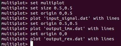
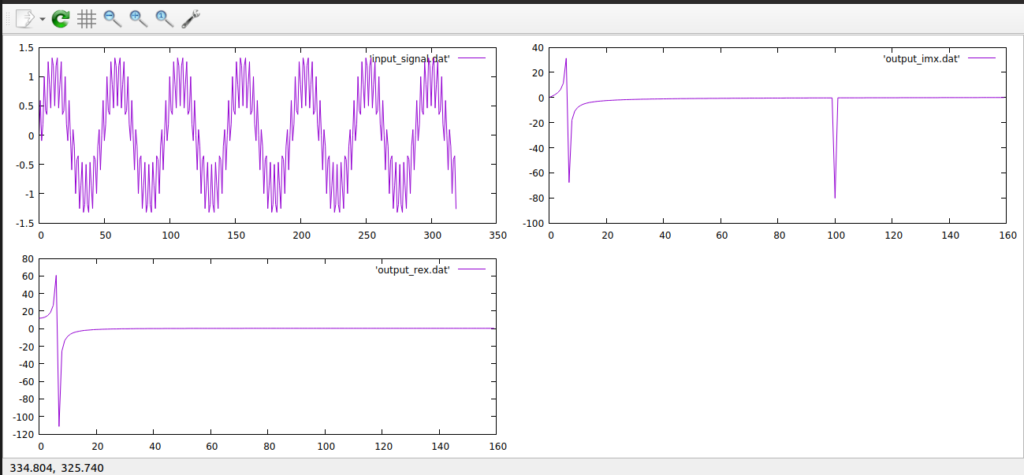
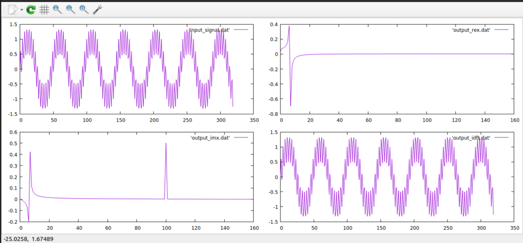
}In order to plot the input signal, the real part and imaginary part of a signal we used a tool called Gnuplot and the command that was used to plot input_signal.dat , output_imx.dat and output_rex.dat are shown below
Inverse Discrete Fourier Transform (IDFT)
in reality, IDFT transforms the frequency domain signal to time Domain signal

![x[i]=\sum_{k=0}^{N/2} Re \bar{X} [k]cos(2\pi k i/N) + \sum_{k=0}^{N/2} Im \bar{X} [k]sin(2\pi k i/N)](https://aneescraftsmanship.com/wp-content/ql-cache/quicklatex.com-3ee5a1097914d19e185dca46ff828bf3_l3.png "Rendered by QuickLaTeX.com")
![\begin{equation*}Re \bar{X}[k]= {\frac{Re X[k]}{N/2} } \end{equation*}](https://aneescraftsmanship.com/wp-content/ql-cache/quicklatex.com-7d551ad58cef7ef3cc6e3cfed90d6c7b_l3.png "Rendered by QuickLaTeX.com")
![\begin{equation*}Im \bar{X}[k]= {-\frac{Im X[k]}{N/2} } \end{equation*}](https://aneescraftsmanship.com/wp-content/ql-cache/quicklatex.com-3a11fe85c4d69379bb1fcc86fcd4ddfc_l3.png "Rendered by QuickLaTeX.com")

![\begin{equation*}Re \bar{X}[0]= {\frac{Re X[0]}{N} } \end{equation*}](https://aneescraftsmanship.com/wp-content/ql-cache/quicklatex.com-ded650d19fefbe0453938989d3e901da_l3.png "Rendered by QuickLaTeX.com")
![\begin{equation*}Re \bar{X}[N/2]= {\frac{Re X[N/2]}{N} } \end{equation*}](https://aneescraftsmanship.com/wp-content/ql-cache/quicklatex.com-0ab9261a49c457a5087678f0af099a32_l3.png "Rendered by QuickLaTeX.com")
#include <stdio.h>
#include <stdlib.h>
#include <math.h>
#define SIG_LENGTH 320
extern float InputSignal_f32_1kHz_15kHz[320];
float Output_REX[SIG_LENGTH/2];
float Output_IMX[SIG_LENGTH/2];
float Output_IDFT[SIG_LENGTH];
float PI =3.14159265359;
void calc_sig_dft(float *sig_src_arr,float *sig_dest_rex_arr, float *sig_dest_imx_arr, int sig_length);
void sig_calc_idft(float *idft_out_arr, float *sig_src_rex_arr,float *sig_src_imx_arr,int idft_length);
int main()
{
     FILE *fptr,*fptr2,*fptr3,*fptr4;
    calc_sig_dft((float *)&InputSignal_f32_1kHz_15kHz[0],(float *)&Output_REX[0],(float *)&Output_IMX[0], (int )SIG_LENGTH);
    sig_calc_idft((float *)&Output_IDFT[0], (float *)&Output_REX[0],(float *)&Output_IMX[0],(int) SIG_LENGTH);
    fptr = fopen("input_signal.dat","w");
    fptr2=fopen ("output_rex.dat","w");
    fptr3=fopen("output_imx.dat","w");
    fptr4=fopen("output_idft.dat","w");
    for(int i=0;i<SIG_LENGTH;i++){
    fprintf(fptr,"\n%f",InputSignal_f32_1kHz_15kHz[i]);
    fprintf(fptr4,"\n%f",Output_IDFT[i]);
    }
    for(int i=0;i<(SIG_LENGTH/2);i++)
    {
        fprintf(fptr2,"\n%f",Output_REX[i]);
        fprintf(fptr3,"\n%f",Output_IMX[i]);
    }
    fclose(fptr);
    fclose(fptr2);
    fclose(fptr3);
    fclose(fptr4);
    return 0;
}
void calc_sig_dft(float *sig_src_arr,float *sig_dest_rex_arr, float *sig_dest_imx_arr, int sig_length)
{
  int i,j,k;
  for(j=0;j<sig_length/2;j++)
  {
      sig_dest_rex_arr[j] =0;
      sig_dest_imx_arr[j] =0;
  }
    for(k=0;k<(sig_length/2);k++)
    {
        for(i=0;i<sig_length;i++)
        {
            sig_dest_rex_arr[k] += sig_src_arr[i]*cos(2*PI*k*i/sig_length);
            sig_dest_imx_arr[k] -= sig_src_arr[i]*sin(2*PI*k*i/sig_length);
        }
    }
}
 void sig_calc_idft(float *idft_out_arr, float *sig_src_rex_arr,float *sig_src_imx_arr,int idft_length)
 {
      int i,k;
      for(k=0;k<idft_length/2;k++)
      {
          sig_src_rex_arr[k] = sig_src_rex_arr[k]/(idft_length/2);
          sig_src_imx_arr[k] = -sig_src_imx_arr[k]/(idft_length/2);
      }
      sig_src_rex_arr[0] = sig_src_rex_arr[0]/2;
      sig_src_rex_arr[idft_length]= sig_src_rex_arr[idft_length]/2;
      for(i=0;i<idft_length;i++)
      {
          idft_out_arr[i]=0;
        }
        for(k=0;k<idft_length/2;k++)
        {
            for(i=0;i<idft_length;i++)
            {
                idft_out_arr[i] += sig_src_rex_arr[k]*cos(2*PI*k*i/idft_length);
                idft_out_arr[i] += sig_src_imx_arr[k]*sin(2*PI*k*i/idft_length);
            }
        }
 }
To plot input_signal.dat, output_rex.dat, output_imx.dat and output_idft.dat we used a tool called Gnuplot, if you don’t know who to use Gnuplot then you can follow this article
Functions to graph by using a tool called Gnuplot
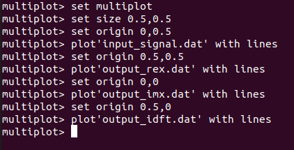
to clarify, the commands that were used in Gnuplot to plot input_signal.dat, output_rex.dat, output_imx.dat and output_idft.dat
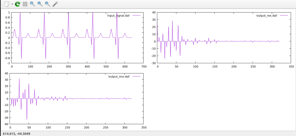
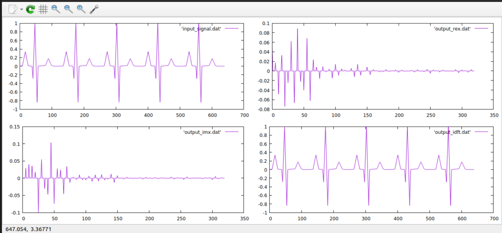
DFT on Electrocardiogram (ECG) Signal
to point out, the Electrocardiogram(ECG) signal is generated in Matlab and you can get that signal source from here —> and the signal source is same for DFT(ECG) and IDFT(ECG)
in a word, the algorithm of DFT and IDFT is used on ECG signal
#include <stdio.h>
#include <stdlib.h>
#include <math.h>
#define SIG_LENGTH 640
extern float _640_points_ecg_[640];
float Output_REX[SIG_LENGTH/2];
float Output_IMX[SIG_LENGTH/2];

void calc_sig_dft(float *sig_src_arr,
                  float *sig_dest_rex_arr,
                  float *sig_dest_imx_arr,
                  int sig_length);

int main()
{
     FILE *fptr1,*fptr2,*fptr3;
    calc_sig_dft((float*) & _640_points_ecg_[0],
                 (float*) & Output_REX[0],
                 (float*) & Output_IMX[0],
                  (int) SIG_LENGTH);

    fptr1 = fopen("input_signal.dat","wt");
    fptr2=fopen ("output_rex.dat","wt");
    fptr3=fopen("output_imx.dat","wt");

    for(int i=0;i<SIG_LENGTH;i++){
    fprintf(fptr1,"\n%f",_640_points_ecg_[i]);
    }
    for(int i=0;i<(SIG_LENGTH/2);i++)
    {
        fprintf(fptr2,"\n%f",Output_REX[i]);
        fprintf(fptr3,"\n%f",Output_IMX[i]);

    }
    fclose(fptr1);
    fclose(fptr2);
    fclose(fptr3);

    return 0;
}
void calc_sig_dft(float *sig_src_arr,float *sig_dest_rex_arr, float *sig_dest_imx_arr, int sig_length)
{
  int i,j,k;
  float PI = 3.14159265359;
  for(j=0;j<sig_length/2;j++)
  {
      sig_dest_rex_arr[j] =0;
      sig_dest_imx_arr[j] =0;
  }
    for(k=0;k<(sig_length/2);k++){
        for(i=0;i<sig_length;i++)
        {
            sig_dest_rex_arr[k] += sig_src_arr[i]*cos(2*PI*k*i/sig_length);
            sig_dest_imx_arr[k] -= sig_src_arr[i]*sin(2*PI*k*i/sig_length);
        }
    }

}
IDFT on Electrocardiogram (ECG) Signal
#include <stdio.h>
#include <stdlib.h>
#include <math.h>
#define SIG_LENGTH 640
extern float _640_points_ecg_[640];
float Output_REX[SIG_LENGTH/2];
float Output_IMX[SIG_LENGTH/2];
float Output_IDFT[SIG_LENGTH];
float PI =3.14159265359;
void calc_sig_dft(float *sig_src_arr,float *sig_dest_rex_arr, float *sig_dest_imx_arr, int sig_length);
void sig_calc_idft(float *idft_out_arr, float *sig_src_rex_arr,float *sig_src_imx_arr,int idft_length);
int main()
{
FILE *fptr,*fptr2,*fptr3,*fptr4;
calc_sig_dft((float *)&_640_points_ecg_[0],(float *)&Output_REX[0],(float *)&Output_IMX[0], (int )SIG_LENGTH);
sig_calc_idft((float *)&Output_IDFT[0], (float *)&Output_REX[0],(float *)&Output_IMX[0],(int) SIG_LENGTH);
fptr = fopen("input_signal.dat","wt");
fptr2=fopen ("output_rex.dat","wt");
fptr3=fopen("output_imx.dat","wt");
fptr4=fopen("output_idft.dat","wt");
for(int i=0;i<SIG_LENGTH;i++){
fprintf(fptr,"\n%f",_640_points_ecg_[i]);
fprintf(fptr4,"\n%f",Output_IDFT[i]);
}
for(int i=0;i<(SIG_LENGTH/2);i++)
{
fprintf(fptr2,"\n%f",Output_REX[i]);
fprintf(fptr3,"\n%f",Output_IMX[i]);
}
fclose(fptr);
fclose(fptr2);
fclose(fptr3);
fclose(fptr4);
return 0;
}
void calc_sig_dft(float *sig_src_arr,float *sig_dest_rex_arr, float *sig_dest_imx_arr, int sig_length)
{
int i,j,k;
for(j=0;j<sig_length/2;j++)
{
sig_dest_rex_arr[j] =0;
sig_dest_imx_arr[j] =0;
}
for(k=0;k<(sig_length/2);k++)
{
for(i=0;i<sig_length;i++)
{
sig_dest_rex_arr[k] += sig_src_arr[i]*cos(2*PI*k*i/sig_length);
sig_dest_imx_arr[k] -= sig_src_arr[i]*sin(2*PI*k*i/sig_length);
}
}
}
void sig_calc_idft(float *idft_out_arr, float *sig_src_rex_arr,float *sig_src_imx_arr,int idft_length)
{
int i,k;
for(k=0;k<idft_length/2;k++)
{
sig_src_rex_arr[k] = sig_src_rex_arr[k]/(idft_length/2);
sig_src_imx_arr[k] = -sig_src_imx_arr[k]/(idft_length/2);
}
sig_src_rex_arr[0] = sig_src_rex_arr[0]/2;
sig_src_rex_arr[idft_length]= sig_src_rex_arr[idft_length]/2;
for(i=0;i<idft_length;i++)
{
idft_out_arr[i]=0;
}
for(k=0;k<idft_length/2;k++)
{
for(i=0;i<idft_length;i++)
{
idft_out_arr[i] += sig_src_rex_arr[k]*cos(2*PI*k*i/idft_length);
idft_out_arr[i] += sig_src_imx_arr[k]*sin(2*PI*k*i/idft_length);
}
}
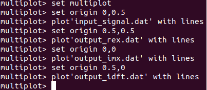
}not to mention, the Gnuplot commands that were used to plot an ECG input signal, the real and imaginary part of an ECG signal and IDFT ECG output signal are shown below
Convolution
in sum, convolution is a mathematical operation to combine two signals to form a third signal and with the help of convolution concept we can build the output of a system for any random input signal if we know the impulse response of a system
![y[n]=x[n]*h[n]=\sum_{-\infty}^{\infty}x[k]*h[n-k]](https://aneescraftsmanship.com/wp-content/ql-cache/quicklatex.com-d590c63d40b5394e432f3c3b95b0849b_l3.png "Rendered by QuickLaTeX.com")
Where
y[n] is an output signal
x[n] is an input signal
h[n] is impulse response
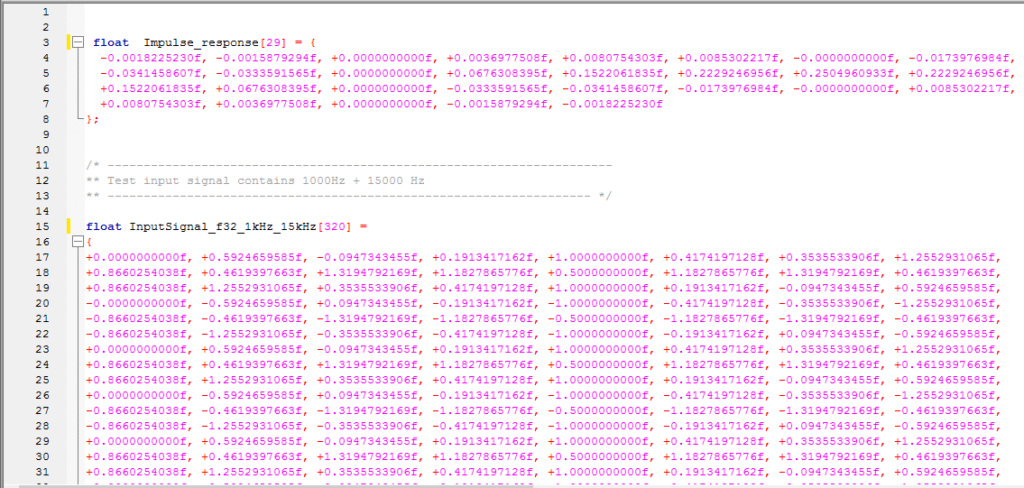
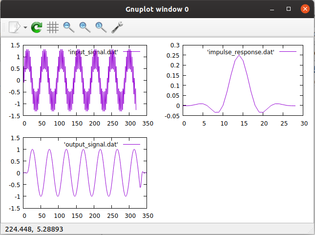
in order to develop a convolution algorithm we used input signal and an impulse response which are generated using matlab, you can get input signal source from here —>and impulse response from here —>
#include <stdio.h>
#include <stdlib.h>
#include <math.h>
#define SIG_LENGTH 320
#define IMP_RSP_LENGTH 29
extern float InputSignal_f32_1kHz_15kHz[SIG_LENGTH];
extern  float Impulse_response[IMP_RSP_LENGTH];
        float Output_signal[SIG_LENGTH+IMP_RSP_LENGTH];
void convolution( float *sig_src_arr,
                  float *sig_dest_arr,
                  float *imp_response_arr,
                  int sig_src_length,
                  int imp_response_length
                 );
int main()
{
    FILE *input_sig_fptr, *imp_rsp_fptr,*output_sig_fptr;
     convolution( (float*) &InputSignal_f32_1kHz_15kHz[0],
                  (float*) &Output_signal[0],
                  (float*) &Impulse_response[0],
                  (int) SIG_LENGTH,
                  (int) IMP_RSP_LENGTH
                 );
    input_sig_fptr = fopen("input_signal.dat","wt");
    imp_rsp_fptr   = fopen ("impulse_response.dat","wt");
    output_sig_fptr = fopen("output_signal.dat","wt");
    for(int i=0;i<SIG_LENGTH;i++)
    {
         fprintf(input_sig_fptr,"\n%f",InputSignal_f32_1kHz_15kHz[i]);
    }
    fclose(input_sig_fptr);
    for(int i=0;i<IMP_RSP_LENGTH;i++)
    {
         fprintf(imp_rsp_fptr,"\n%f",Impulse_response[i]);
    }
    fclose(imp_rsp_fptr);
     for(int i=0;i<SIG_LENGTH+IMP_RSP_LENGTH;i++)
     {
         fprintf(output_sig_fptr,"\n%f",Output_signal[i]);
     }
     fclose(output_sig_fptr);
    return 0;
}

void convolution( float *sig_src_arr,
                  float *sig_dest_arr,
                  float *imp_response_arr,
                  int sig_src_length,
                  int imp_response_length
                 )
{
    int i,j;
      for(i=0;i<sig_src_length;i++)
      {
          for(j=0;j<imp_response_length;j++)
          {
              sig_dest_arr[i+j] += sig_src_arr[i]*imp_response_arr[j];
          }
      }
}
To plot input .dat file and output.dat and impulse .dat we used a tool called Gnuplot, if you don’t know who to use Gnuplot then you can follow this article
Functions to graph by using a tool called Gnuplot
as can be seen, the commands that were used in Gnuplot to plot input.dat, output.dat and impulse.dat
Leave a Reply